
Structure optimization#
The optimization algorithms can be roughly divided into local optimization algorithms which find a nearby local minimum and global optimization algorithms that try to find the global minimum (a much harder task).
Most optimization algorithms available in ASE inherit the following
Optimizer base-class.
- class ase.optimize.optimize.Optimizer(atoms: Atoms, restart: str | Path | None = None, logfile: IO | str | Path | None = None, trajectory: str | Path | None = None, append_trajectory: bool = False, **kwargs)[source]#
Base-class for all structure optimization classes.
- Parameters:
atoms (
Atoms) – The Atoms object to relax.restart (str | Path | None) – Filename for restart file. Default value is None.
logfile (file object, Path, or str) – If logfile is a string, a file with that name will be opened. Use ‘-’ for stdout.
trajectory (Trajectory object, Path, or str) – Attach trajectory object. If trajectory is a string a Trajectory will be constructed. Use None for no trajectory.
append_trajectory (bool) – Appended to the trajectory file instead of overwriting it.
kwargs (dict, optional) – Extra arguments passed to
Dynamics.
Note
Optimizer classes themselves optimize only
internal atomic positions.
Cell volume and shape can also be optimized in combination with Filter
classes. (See Filters for details.)
Local optimization#
The local optimization algorithms available in ASE are: BFGS,
BFGSLineSearch, LBFGS, LBFGSLineSearch,
GoodOldQuasiNewton, CellAwareBFGS, RFO,
GPMin, MDMin, FIRE and FIRE2/ABC-FIRE.
See also
Performance test
for all ASE local optimizers with GPAW.
Figs. S7-10 in this SI from 2025
also shows performance tests with ML potentials.
MDMin and FIRE both use Newtonian dynamics with added
friction, to converge to an energy minimum, whereas the others are of
the quasi-Newton type, where the forces of consecutive steps are used
to dynamically update a Hessian describing the curvature of the
potential energy landscape. You can use the QuasiNewton synonym
for BFGSLineSearch because this algorithm is in many cases the optimal
of the quasi-Newton algorithms.
All of the local optimizer classes have the following structure:
class Optimizer:
    def __init__(self, atoms, restart=None, logfile=None):
    def run(self, fmax=0.05, steps=100000000):
    def get_number_of_steps():
The convergence criterion is that the force on all individual atoms should be less than fmax:
BFGS#
- class ase.optimize.BFGS(atoms: Atoms, restart: str | Path | None = None, logfile: IO | str | Path | None = '-', trajectory: str | Path | None = None, append_trajectory: bool = False, maxstep: float | None = None, alpha: float | None = None, **kwargs)[source]#
BFGS optimizer.
- Parameters:
atoms (
Atoms) – The Atoms object to relax.restart (str | Path | None) – JSON file used to store hessian matrix. If set, file with such a name will be searched and hessian matrix stored will be used, if the file exists.
trajectory (str or Path) – Trajectory file used to store optimisation path.
logfile (file object, Path, or str) – If logfile is a string, a file with that name will be opened. Use ‘-’ for stdout.
maxstep (float) – Used to set the maximum distance an atom can move per iteration (default value is 0.2 Å).
alpha (float) – Initial guess for the Hessian (curvature of energy surface). A conservative value of 70.0 is the default, but number of needed steps to converge might be less if a lower value is used. However, a lower value also means risk of instability.
kwargs (dict, optional) – Extra arguments passed to
Optimizer.
Examples
The BFGS object is one of the minimizers in the ASE package. The below script uses BFGS to optimize the structure of a water molecule, starting with the experimental geometry:
>>> from ase import Atoms
>>> from ase.optimize import BFGS
>>> from ase.calculators.emt import EMT
>>> import numpy as np
>>> d = 0.9575
>>> t = np.pi / 180 * 104.51
>>> system = Atoms('H2O',
... positions=[(d, 0, 0),
... (d * np.cos(t), d * np.sin(t), 0),
... (0, 0, 0)],
... calculator=EMT())
>>> dyn = BFGS(system)
>>> dyn.run(fmax=0.05)
      Step     Time          Energy          fmax
BFGS:    0 ...        2.769632        8.609090
BFGS:    1 ...        1.930507        1.641499
BFGS:    2 ...        1.884227        0.535354
BFGS:    3 ...        1.879314        0.049628
...
The columns are the solver name, step number, clock time, potential energy (eV), and maximum force (eV/Å).
When doing structure optimization, it is useful to write the trajectory to a file, so that the progress of the optimization run can be followed during or after the run:
dyn = BFGS(system, trajectory='H2O.traj')
dyn.run(fmax = 0.05)
Use the command ase gui H2O.traj to see what is going on (more here:
ase.gui). The trajectory file can also be accessed using the
module ase.io.trajectory.
The attach method takes an optional argument interval = n that can be
used to tell the structure optimizer object to write the configuration to
the trajectory file only every n steps:
from ase.optimize import BFGS
from ase.io import Trajectory
...
dyn = BFGS(system, trajectory='H2O.traj')
traj = Trajectory('H2O.traj', 'w', system)
dyn.attach(traj.write, interval = 2)
dyn.run(fmax = 0.05)
During a structure optimization, the BFGS and LBFGS optimizers use two quantities to decide where to move the atoms on each step, e.g.:
the forces on each atom, as returned by the associated
Calculatorobjectthe Hessian matrix, i.e. the matrix of second derivatives \(\frac{\partial^2 E}{\partial x_i \partial x_j}\) of the total energy with respect to nuclear coordinates.
If the atoms are close to the minimum, such that the potential energy surface is locally quadratic, the Hessian and forces accurately determine the required step to reach the optimal structure. The Hessian is very expensive to calculate a priori, so instead the algorithm estimates it by means of an initial guess which is adjusted along the way depending on the information obtained on each step of the structure optimization.
It is frequently practical to restart or continue a structure
optimization with a geometry obtained from a previous relaxation.
Aside from the geometry, the Hessian of the previous run can and
should be retained for the second run. Use the restart keyword to
specify a file in which to save the Hessian:
dyn = BFGS(atoms=system, trajectory = 'H2O.traj', restart = 'H2O.json')
This will create an optimizer which saves the Hessian to
'H2O.json (using the Python json module) on each
step. If the file already exists, the Hessian will also be
initialized from that file.
The trajectory file can also be used to restart a structure optimization, since it contains the history of all forces and positions, and thus whichever information about the Hessian was assembled so far:
from ase.io import read
from ase.calculators.emt import EMT
from ase.optimize import BFGS

system = read('H2O.traj')
system.calc = EMT()
dyn2 = BFGS(system, trajectory='part2.traj')
dyn2.replay_trajectory('H2O.traj')
dyn2.run(fmax = 0.01)
replay_trajectory will read through each iteration stored in
H2O.traj, performing adjustments to the Hessian as appropriate.
Setting dyn.run(fmax = 0.01) then continues the trajectory calculation from
the stored iterations.
Note that the stored steps will not be written to H2O.traj, i.e.,
H2O.traj will only contain the steps from the continued trajectory
calculation. Be careful not to use the same filename for H2O.traj and
part2.traj to avoid overwriting the previous iterations.
If restarting with more than one previous trajectory file, use
Graphical user interface (GUI) to concatenate them into a single trajectory file first:
$ ase gui H2O.traj part2.traj -o history.traj
The file history.traj will then contain all necessary
information.
When switching between different types of optimizers, e.g. between
BFGS and LBFGS, the JSON-files specified by the
restart keyword are not compatible, but the Hessian can still be
retained by replaying the trajectory as above.
LBFGS#
LBFGS is the limited memory version of the BFGS algorithm, where
the inverse of Hessian matrix is updated instead of the Hessian
itself. Two ways exist for determining the atomic
step: Standard LBFGS and LBFGSLineSearch. For the
first one, both the directions and lengths of the atomic steps
are determined by the approximated Hessian matrix. While for the
latter one, the approximated Hessian matrix is only used to find
out the directions of the line searches and atomic steps, the
step lengths are determined by the forces.
The syntax for a structure optimisation with LBFGS and LBGGSLineSearch
follow the format of the BFGS.
- class ase.optimize.LBFGS(atoms: Atoms, restart: str | None = None, logfile: IO | str = '-', trajectory: str | None = None, maxstep: float | None = None, memory: int = 100, damping: float = 1.0, alpha: float = 70.0, use_line_search: bool = False, **kwargs)[source]#
Limited memory BFGS optimizer.
A limited memory version of the BFGS algorithm. Unlike the BFGS algorithm used in bfgs.py, the inverse of Hessian matrix is updated. The inverse Hessian is represented only as a diagonal matrix to save memory
- Parameters:
atoms (
Atoms) – The Atoms object to relax.restart (str) – JSON file used to store vectors for updating the inverse of Hessian matrix. If set, file with such a name will be searched and information stored will be used, if the file exists.
logfile (file object or str) – If logfile is a string, a file with that name will be opened. Use ‘-’ for stdout.
trajectory (string) – Trajectory file used to store optimisation path.
maxstep (float) – How far is a single atom allowed to move. This is useful for DFT calculations where wavefunctions can be reused if steps are small. Default is 0.2 Angstrom.
memory (int) – Number of steps to be stored. Default value is 100. Three numpy arrays of this length containing floats are stored.
damping (float) – The calculated step is multiplied with this number before added to the positions.
alpha (float) – Initial guess for the Hessian (curvature of energy surface). A conservative value of 70.0 is the default, but number of needed steps to converge might be less if a lower value is used. However, a lower value also means risk of instability.
kwargs (dict, optional) – Extra arguments passed to
Optimizer.
Examples
>>> from ase import Atoms
>>> from ase.optimize import LBFGS
>>> from ase.calculators.emt import EMT
...
>>> system = Atoms(
... 'N2',
... positions = [(0.0, 0.0, 0.0), (0.0, 0.0, 1.1)],
... calculator=EMT()
... )
>>> dyn = LBFGS(system)
>>> dyn.run(fmax=0.05)
       Step     Time          Energy          fmax
LBFGS:    0 ...        0.440344        3.251800
LBFGS:    1 ...        0.264361        0.347497
LBFGS:    2 ...        0.262860        0.080535
LBFGS:    3 ...        0.262777        0.001453
...
GoodOldQuasiNewton#
While GOQN is an “old” optimizer in the history of ASE, it can be very effective and often converges in fewer steps than newer optimizers. The GOQN is used with a similar syntax as the BFGS.
- class ase.optimize.GoodOldQuasiNewton(atoms: Atoms, restart: str | None = None, logfile: IO | str = '-', trajectory: str | None = None, fmax=None, converged=None, hessianupdate: str = 'BFGS', hessian=None, forcemin: bool = True, verbosity: bool = False, maxradius: float | None = None, diagonal: float = 20.0, radius: float | None = None, transitionstate: bool = False, **kwargs)[source]#
- Parameters:
atoms (
Atoms) – The Atoms object to relax.restart (str) – File used to store hessian matrix. If set, file with such a name will be searched and hessian matrix stored will be used, if the file exists.
trajectory (str) – File used to store trajectory of atomic movement.
maxstep (float) – Used to set the maximum distance an atom can move per iteration (default value is 0.2 Angstroms).
- logfile: file object or str
If logfile is a string, a file with that name will be opened. Use ‘-’ for stdout.
- kwargsdict, optional
Extra arguments passed to
Optimizer.
Examples
>>> from ase import Atoms
>>> from ase.optimize import LBFGS
>>> from ase.calculators.emt import EMT
...
>>> system = Atoms(
... 'N2',
... positions = [(0.0, 0.0, 0.0), (0.0, 0.0, 1.1)],
... calculator=EMT()
... )
>>> dyn = LBFGS(system)
>>> dyn.run(fmax=0.05)
CellAwareBFGS#
CellAwareBFGS requires a UnitCellFilter (usually the
FrechetCellFilter is the best choice) and can use additional
information about the system (bulk modulus, Posson ratio) to inform the
optimization process.
The CellAwareBFGS can be used as follows:
from ase.build import bulk
from ase.calculators.emt import EMT
from ase.filters import FrechetCellFilter
from ase.optimize.cellawarebfgs import CellAwareBFGS
from ase.units import GPa

atoms = bulk('Au')

atoms.calc = EMT()
dyn = CellAwareBFGS(
        FrechetCellFilter(atoms, exp_cell_factor=1.0),
        alpha=70, # suppress-ratio for elastic tensor calculation
        bulk_modulus = 100 * GPa,
        poisson_ratio = 0.37,
        long_output=True,
    )
dyn.run(fmax=0.005)
RFO#
- class ase.optimize.RFO(*args, damping: float | None = None, eigsh_maxiter: int | None = None, **kwargs)[source]#
RFO (Rational Function Optimizer) combined with BFGS-based Hessian updates.
RFO will take quasi-Newton-like steps in quadratic regime and rational function damped steps outside of it. The
dampingfactor determines the transition threshold between the regimes.Read about this algorithm here:
A. Banerjee, N. Adams, J. Simons, R. Shepard,J. Phys. Chem. 1985, 89, 52-57.Note that
dampingis the reciprocal of coordinate scale \(a\) from the reference.- Parameters:
*args – Positional arguments passed to
BFGS.damping (float) – Determines transition threshold between quasi-Newton-like and rational function damped steps. The larger the value, the larger and stronger the damped regime. (default is 1.0 Å^-1).
eigsh_maxiter (int) – Maximum number of eigsh iterations done before falling back to eigh for solving the RFO step.
**kwargs – Keyword arguments passed to
BFGS.
Examples
>>> from ase import Atoms
>>> from ase.optimize import RFO
>>> from ase.calculators.emt import EMT
...
>>> system = Atoms(
... 'N2',
... positions = [(0.0, 0.0, 0.0), (0.0, 0.0, 1.1)],
... calculator=EMT()
... )
>>> dyn = RFO(system)
>>> dyn.run(fmax=0.05)
     Step     Time          Energy          fmax
RFO:    0 ...        0.440344        3.251800
RFO:    1 ...        0.264502        0.362456
RFO:    2 ...        0.262867        0.084092
RFO:    3 ...        0.262777        0.001583
...
GPMin#
The GPMin (Gaussian Process minimizer) produces a model for the Potential Energy Surface using the information about the potential energies and the forces of the configurations it has already visited and uses it to speed up BFGS local minimzations.
Read more about this algorithm here:
Estefanía Garijo del Río, Jens Jørgen Mortensen, Karsten W. JacobsenPhysical Review B, Vol. 100, 104103 (2019)
Warning
The memory of the optimizer scales as O(n²N²) where N is the number of atoms and n the number of steps. If the number of atoms is sufficiently high, this may cause a memory issue. This class prints a warning if the user tries to run GPMin with more than 100 atoms in the unit cell.
- class ase.optimize.GPMin(atoms, restart=None, logfile='-', trajectory=None, prior=None, kernel=None, noise=None, weight=None, scale=None, batch_size=None, bounds=None, update_prior_strategy='maximum', update_hyperparams=False, **kwargs)[source]#
Optimize atomic positions using GPMin algorithm, which uses both potential energies and forces information to build a PES via Gaussian Process (GP) regression and then minimizes it.
Default behaviour:#
The default values of the scale, noise, weight, batch_size and bounds parameters depend on the value of update_hyperparams. In order to get the default value of any of them, they should be set up to None. Default values are:
- update_hyperparams = True
scale : 0.3 noise : 0.004 weight: 2. bounds: 0.1 batch_size: 1
- update_hyperparams = False
scale : 0.4 noise : 0.005 weight: 1. bounds: irrelevant batch_size: irrelevant
- param atoms:
The Atoms object to relax.
- type atoms:
- param restart:
JSON file used to store the training set. If set, file with such a name will be searched and the data in the file incorporated to the new training set, if the file exists.
- type restart:
str
- param logfile:
If logfile is a string, a file with that name will be opened. Use ‘-’ for stdout
- type logfile:
file object or str
- param trajectory:
File used to store trajectory of atomic movement.
- type trajectory:
str
- param prior:
Prior for the GP regression of the PES surface See ase.optimize.gpmin.prior If prior is None, then it is set as the ConstantPrior with the constant being updated using the update_prior_strategy specified as a parameter
- type prior:
Prior object or None
- param kernel:
Kernel for the GP regression of the PES surface See ase.optimize.gpmin.kernel If kernel is None the SquaredExponential kernel is used. Note: It needs to be a kernel with derivatives!!!!!
- type kernel:
Kernel object or None
- param noise:
Regularization parameter for the Gaussian Process Regression.
- type noise:
float
- param weight:
Prefactor of the Squared Exponential kernel. If update_hyperparams is False, changing this parameter has no effect on the dynamics of the algorithm.
- type weight:
float
- param update_prior_strategy:
Strategy to update the constant from the ConstantPrior when more data is collected. It does only work when Prior = None
- options:
‘maximum’: update the prior to the maximum sampled energy ‘init’ : fix the prior to the initial energy ‘average’: use the average of sampled energies as prior
- type update_prior_strategy:
str
- param scale:
scale of the Squared Exponential Kernel
- type scale:
float
- param update_hyperparams:
Update the scale of the Squared exponential kernel every batch_size-th iteration by maximizing the marginal likelihood.
- type update_hyperparams:
bool
- param batch_size:
Number of new points in the sample before updating the hyperparameters. Only relevant if the optimizer is executed in update_hyperparams mode: (update_hyperparams = True)
- type batch_size:
int
- param bounds:
Set bounds to the optimization of the hyperparameters. Let t be a hyperparameter. Then it is optimized under the constraint (1-bound)*t_0 <= t <= (1+bound)*t_0 where t_0 is the value of the hyperparameter in the previous step. If bounds is False, no constraints are set in the optimization of the hyperparameters.
- type bounds:
float, 0<bounds<1
- param kwargs:
Extra arguments passed to
Optimizer.- type kwargs:
dict, optional
- param .. warning::
The memory of the optimizer scales as O(n²N²) where: N is the number of atoms and n the number of steps. If the number of atoms is sufficiently high, this may cause a memory issue. This class prints a warning if the user tries to run GPMin with more than 100 atoms in the unit cell.
Examples
>>> from ase import Atoms
>>> from ase.calculators.emt import EMT
>>> from ase.optimize.gpmin.gpmin import GPMin
...
>>> system = Atoms(
... 'N2',
... positions = [(0.0, 0.0, 0.0), (0.0, 0.0, 1.1)],
... calculator=EMT()
... )
>>> dyn = GPMin(system)
>>> dyn.run(fmax=0.05)
       Step     Time          Energy          fmax
GPMin:    0 ...        0.440344        3.251800
GPMin:    1 ...        0.357046        2.961912
GPMin:    2 ...        0.262953        0.116630
GPMin:    3 ...        0.262777        0.004907
...
FIRE#
Read about this algorithm here:
Erik Bitzek, Pekka Koskinen, Franz Gähler, Michael Moseler, and Peter GumbschPhysical Review Letters, Vol. 97, 170201 (2006)
- class ase.optimize.FIRE(atoms: Atoms, restart: str | None = None, logfile: IO | str = '-', trajectory: str | None = None, dt: float = 0.1, maxstep: float | None = None, maxmove: float | None = None, dtmax: float = 1.0, Nmin: int = 5, finc: float = 1.1, fdec: float = 0.5, astart: float = 0.1, fa: float = 0.99, a: float = 0.1, downhill_check: bool = False, position_reset_callback: Callable | None = None, **kwargs)[source]#
- Parameters:
atoms (
Atoms) – The Atoms object to relax.restart (str) – JSON file used to store hessian matrix. If set, file with such a name will be searched and hessian matrix stored will be used, if the file exists.
logfile (file object or str) – If logfile is a string, a file with that name will be opened. Use ‘-’ for stdout.
trajectory (str) – Trajectory file used to store optimisation path.
dt (float) – Initial time step. Defualt value is 0.1
maxstep (float) – Used to set the maximum distance an atom can move per iteration (default value is 0.2).
dtmax (float) – Maximum time step. Default value is 1.0
Nmin (int) – Number of steps to wait after the last time the dot product of the velocity and force is negative (P in The FIRE article) before increasing the time step. Default value is 5.
finc (float) – Factor to increase the time step. Default value is 1.1
fdec (float) – Factor to decrease the time step. Default value is 0.5
astart (float) – Initial value of the parameter a. a is the Coefficient for mixing the velocity and the force. Called alpha in the FIRE article. Default value 0.1.
fa (float) – Factor to decrease the parameter alpha. Default value is 0.99
a (float) – Coefficient for mixing the velocity and the force. Called alpha in the FIRE article. Default value 0.1.
downhill_check (bool) – Downhill check directly compares potential energies of subsequent steps of the FIRE algorithm rather than relying on the current product v*f that is positive if the FIRE dynamics moves downhill. This can detect numerical issues where at large time steps the step is uphill in energy even though locally v*f is positive, i.e. the algorithm jumps over a valley because of a too large time step.
position_reset_callback (function(atoms, r, e, e_last)) – Function that takes current atoms object, an array of position r that the optimizer will revert to, current energy e and energy of last step e_last. This is only called if e > e_last.
kwargs (dict, optional) – Extra arguments passed to
Optimizer.deprecated: (..) – 3.19.3: Use of
maxmoveis deprecated; please usemaxstep.
Examples
>>> from ase import Atoms
>>> from ase.optimize import FIRE
>>> from ase.calculators.emt import EMT
...
>>> system = Atoms(
... 'N2',
... positions = [(0.0, 0.0, 0.0), (0.0, 0.0, 1.1)],
... calculator=EMT()
... )
>>> dyn = FIRE(system, dtmax = 1.0, dt = 2.0)
>>> dyn.run(fmax=0.05)
      Step     Time          Energy          fmax
FIRE:    0 ...        0.440344        3.251800
FIRE:    1 ...        1.076992       10.112458
FIRE:    2 ...        0.440344        3.251800
FIRE:    3 ...        1.076992       10.112458
FIRE:    4 ...        0.440344        3.251800
FIRE:    5 ...        0.262779        0.013728
...
FIRE2.0 / ABC-FIRE#
FIRE2.0 and ABC-FIRE are implemented by the same class, with the latter enabled by the use_abc parameter.
J. Guénolé, W.G. Nöhring, A. Vaid, F. Houllé, Z. Xie, A. Prakash, E. Bitzek,Comput. Mater. Sci. 175 (2020) 109584.S. Echeverri Restrepo, P. Andric,Comput. Mater. Sci. 218 (2023) 111978.
- class ase.optimize.FIRE2(atoms: Atoms, restart: str | None = None, logfile: IO | str = '-', trajectory: str | None = None, dt: float = 0.1, maxstep: float = 0.2, dtmax: float = 1.0, dtmin: float = 0.002, Nmin: int = 20, finc: float = 1.1, fdec: float = 0.5, astart: float = 0.25, fa: float = 0.99, position_reset_callback: Callable | None = None, use_abc: bool | None = False, **kwargs)[source]#
- Parameters:
atoms (
Atoms) – The Atoms object to relax.restart (str) – JSON file used to store hessian matrix. If set, file with such a name will be searched and hessian matrix stored will be used, if the file exists.
logfile (file object or str) – If logfile is a string, a file with that name will be opened. Use ‘-’ for stdout.
trajectory (str) – Trajectory file used to store optimisation path.
dt (float) – Initial time step. Defualt value is 0.1
maxstep (float) – Used to set the maximum distance an atom can move per iteration (default value is 0.2). Note that for ABC-FIRE the check is done independently for each cartesian direction.
dtmax (float) – Maximum time step. Default value is 1.0
dtmin (float) – Minimum time step. Default value is 2e-3
Nmin (int) – Number of steps to wait after the last time the dot product of the velocity and force is negative (P in The FIRE article) before increasing the time step. Default value is 20.
finc (float) – Factor to increase the time step. Default value is 1.1
fdec (float) – Factor to decrease the time step. Default value is 0.5
astart (float) – Initial value of the parameter a. a is the Coefficient for mixing the velocity and the force. Called alpha in the FIRE article. Default value 0.25.
fa (float) – Factor to decrease the parameter alpha. Default value is 0.99
position_reset_callback (function(atoms, r, e, e_last)) – Function that takes current atoms object, an array of position r that the optimizer will revert to, current energy e and energy of last step e_last. This is only called if e > e_last.
use_abc (bool) – If True, the Accelerated Bias-Corrected FIRE algorithm is used (ABC-FIRE). Default value is False.
kwargs (dict, optional) – Extra arguments passed to
Optimizer.
Examples
>>> from ase import Atoms
>>> from ase.optimize import FIRE2
>>> from ase.calculators.emt import EMT
...
>>> system = Atoms(
... 'N2',
... positions = [(0.0, 0.0, 0.0), (0.0, 0.0, 1.1)],
... calculator=EMT()
... )
>>> fire_parameters = {
... 'dt': 0.5,
... 'maxstep': 0.2,
... 'dtmax': 1.0,
... 'Nmin': 20,
... 'finc': 1.1,
... 'fdec': 0.5,
... 'astart': 0.25,
... 'fa': 0.99,
... }
>>> dyn = FIRE2(system, use_abc=True, **fire_parameters)
>>> dyn.run(fmax=0.05)
       Step     Time          Energy          fmax
FIRE2:    0 ...        0.440344        3.251800
FIRE2:    1 ...        2.859671       21.028202
FIRE2:    2 ...        0.875141        5.281651
FIRE2:    3 ...        2.859671       21.028202
FIRE2:    4 ...        0.668117        4.546505
FIRE2:    5 ...        0.311649        1.823901
FIRE2:    6 ...        0.262793        0.035743
...
MDMin#
The MDmin algorithm is a modification of the usual velocity-Verlet molecular dynamics algorithm. Newtons second law is solved numerically, but after each time step the dot product between the forces and the momenta is checked. If it is zero, the system has just passed through a (local) minimum in the potential energy, the kinetic energy is large and about to decrease again. At this point, the momentum is set to zero. Unlike a “real” molecular dynamics, the masses of the atoms are not used, instead all masses are set to one.
The MDmin algorithm exists in two flavors, one where each atom is tested and stopped individually, and one where all coordinates are treated as one long vector, and all momenta are set to zero if the dot product between the momentum vector and force vector (both of length 3N) is zero. This module implements the latter version.
Although the algorithm is primitive, it performs very well because it takes advantage of the physics of the problem. Once the system is so near the minimum that the potential energy surface is approximately quadratic it becomes advantageous to switch to a minimization method with quadratic convergence, such as Conjugate Gradient or Quasi Newton.
- class ase.optimize.MDMin(atoms: Atoms, restart: str | None = None, logfile: IO | str = '-', trajectory: str | None = None, dt: float | None = None, maxstep: float | None = None, **kwargs)[source]#
- Parameters:
atoms (
Atoms) – The Atoms object to relax.restart (str) – JSON file used to store hessian matrix. If set, file with such a name will be searched and hessian matrix stored will be used, if the file exists.
trajectory (str) – Trajectory file used to store optimisation path.
logfile (str) – Text file used to write summary information.
dt (float) – Time step for integrating the equation of motion.
maxstep (float) – Spatial step limit in Angstrom. This allows larger values of dt while being more robust to instabilities in the optimization.
kwargs (dict, optional) – Extra arguments passed to
Optimizer.
Examples
>>> from ase import Atoms
>>> from ase.optimize import MDMin
>>> from ase.calculators.emt import EMT
...
>>> system = Atoms(
... 'N2',
... positions = [(0.0, 0.0, 0.0), (0.0, 0.0, 1.1)],
... calculator=EMT()
... )
>>> dyn = MDMin(system)
>>> dyn.run(fmax=0.05)
       Step     Time          Energy          fmax
MDMin:    0 ...        0.440344        3.251800
MDMin:    1 ...        0.278778        1.160079
MDMin:    2 ...        0.269160        0.689054
MDMin:    3 ...        0.264472        0.368254
MDMin:    4 ...        0.263357        0.211246
MDMin:    5 ...        0.262951        0.117040
MDMin:    6 ...        0.262833        0.066207
MDMin:    7 ...        0.262795        0.037033
...
SciPy optimizers#
SciPy provides a number of optimizers. An interface module for a couple of these have been written for ASE. Most notable are the optimizers SciPyFminBFGS and SciPyFminCG.
- class ase.optimize.sciopt.SciPyFminCG#
- class ase.optimize.sciopt.SciPyFminBFGS(atoms: Atoms, logfile: IO | str = '-', trajectory: str | None = None, callback_always: bool = False, alpha: float = 70.0, **kwargs)[source]#
Quasi-Newton method (Broydon-Fletcher-Goldfarb-Shanno)
Initialize object
- Parameters:
atoms (
Atoms) – The Atoms object to relax.trajectory (str) – Trajectory file used to store optimisation path.
logfile (file object or str) – If logfile is a string, a file with that name will be opened. Use ‘-’ for stdout.
callback_always (bool) – Should the callback be run after each force call (also in the linesearch)
alpha (float) – Initial guess for the Hessian (curvature of energy surface). A conservative value of 70.0 is the default, but number of needed steps to converge might be less if a lower value is used. However, a lower value also means risk of instability.
kwargs (dict, optional) – Extra arguments passed to
Optimizer.
Examples
SciPy provides a number of optimizers. An interface module for a couple of these have been written for ASE. Most notable are the optimizers SciPyFminBFGS and SciPyFminCG. These can be imported as:
>>> from ase.optimize.sciopt import SciPyFminBFGS, SciPyFminCG
>>> from ase.calculators.emt import EMT
>>> from ase import Atoms
>>> system = Atoms(
... 'N2',
... positions = [(0.0, 0.0, 0.0), (0.0, 0.0, 1.1)],
... calculator=EMT()
... )
>>> # The optimizers are called with the regular syntax, e.g.:
>>> dyn = SciPyFminBFGS(system)
>>> dyn.run(fmax=0.05)
               Step     Time          Energy          fmax
SciPyFminBFGS:    0 ...        0.440344        3.251800
SciPyFminBFGS:    1 ...        0.264361        0.347497
SciPyFminBFGS:    2 ...        0.262860        0.080535
SciPyFminBFGS:    3 ...        0.262777        0.001453
...
BFGSLineSearch#
BFGSLineSearch is the BFGS algorithm with a line search mechanism that enforces the step taken fulfills the Wolfe conditions, so that the energy and absolute value of the force decrease monotonically. Like the LBFGS algorithm the inverse of the Hessian Matrix is updated.
Note
In many of the examples, tests, exercises and tutorials,
QuasiNewton is used – it is a synonym for BFGSLineSearch.
The BFGSLineSearch algorithm is not compatible with nudged elastic band calculations.
- class ase.optimize.BFGSLineSearch(atoms: Atoms, restart: str | None = None, logfile: IO | str = '-', maxstep: float | None = None, trajectory: str | None = None, c1: float = 0.23, c2: float = 0.46, alpha: float = 10.0, stpmax: float = 50.0, **kwargs)[source]#
Optimize atomic positions in the BFGSLineSearch algorithm, which uses both forces and potential energy information.
- Parameters:
atoms (
Atoms) – The Atoms object to relax.restart (str) – JSON file used to store hessian matrix. If set, file with such a name will be searched and hessian matrix stored will be used, if the file exists.
trajectory (str) – Trajectory file used to store optimisation path.
maxstep (float) – Used to set the maximum distance an atom can move per iteration (default value is 0.2 Angstroms).
logfile (file object or str) – If logfile is a string, a file with that name will be opened. Use ‘-’ for stdout.
kwargs (dict, optional) – Extra arguments passed to
Optimizer.
Examples
>>> from ase import Atoms
>>> from ase.optimize.bfgslinesearch import BFGSLineSearch
>>> from ase.calculators.emt import EMT
...
>>> system = Atoms(
... 'N2',
... positions = [(0.0, 0.0, 0.0), (0.0, 0.0, 1.1)],
... calculator=EMT()
... )
>>> dyn = BFGSLineSearch(system)
>>> dyn.run(fmax=0.05)
                Step[ FC]     Time          Energy          fmax
BFGSLineSearch:    0[  0] ...        0.440344       3.2518
BFGSLineSearch:    1[  2] ...        0.265703       0.4702
BFGSLineSearch:    2[  3] ...        0.262932       0.1103
BFGSLineSearch:    3[  4] ...        0.262777       0.0027
...
- ase.optimize.QuasiNewton#
alias of
BFGSLineSearch
Preconditioned optimizers#
Preconditioners can speed up optimization approaches by incorporating information about the local bonding topology into a redefined metric through a coordinate transformation. Preconditioners are problem dependent, but the general purpose-implementation in ASE provides a basis that can be adapted to achieve optimized performance for specific applications.
While the approach is general, the implementation is specific to a
given optimizer: currently LBFGS and FIRE can be preconditioned using
the ase.optimize.precon.lbfgs.PreconLBFGS and
ase.optimize.precon.fire.PreconFIRE classes, respectively.
You can read more about the theory and implementation here:
D. Packwood, J.R. Kermode; L. Mones, N. Bernstein, J. Woolley, N. Gould, C. Ortner and G. CsányiJ. Chem. Phys. 144, 164109 (2016).
Tests with a variety of solid-state systems using both DFT and classical
interatomic potentials driven though ASE calculators show speedup factors of up
to an order of magnitude for preconditioned L-BFGS over standard L-BFGS, and the
gain grows with system size. Precomputations are performed to automatically
estimate all parameters required. A linesearch based on enforcing only the first
Wolff condition (i.e. the Armijo sufficient descent condition) is also provided
in ase.utils.linesearcharmijo; this typically leads to a further speed up
when used in conjunction with the preconditioner.
For small systems, unless they are highly ill-conditioned due to large
variations in bonding stiffness, it is unlikely that preconditioning provides a
performance gain, and standard BFGS and LBFGS should be preferred. Therefore,
for systems with fewer than 100 atoms, PreconLBFGS reverts to standard LBFGS.
Preconditioning can be enforces with the keyword argument precon.
The preconditioned L-BFGS method implemented in ASE does not require external
dependencies, but the scipy.sparse module can be used for efficient
sparse linear algebra, and the matscipy package is used for fast
computation of neighbour lists if available. The PyAMG package can be used to
efficiently invert the preconditioner using an adaptive multigrid method.
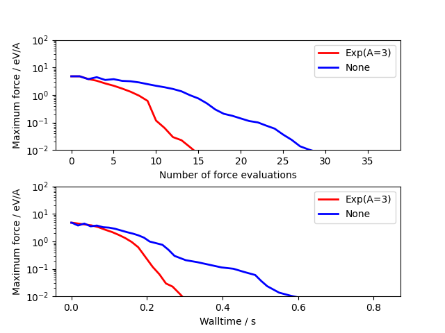
Usage is very similar to the standard optimizers. The example below compares
unpreconditioned LBGFS with the default Exp preconditioner for a 3x3x3 bulk
cube of copper containing a vacancy:
import numpy as np
from ase.build import bulk
from ase.calculators.emt import EMT
from ase.optimize.precon import Exp, PreconLBFGS

from ase.calculators.loggingcalc import LoggingCalculator
import matplotlib as mpl
mpl.use('Agg')
import matplotlib.pyplot as plt

a0 = bulk('Cu', cubic=True)
a0 *= [3, 3, 3]
del a0[0]
a0.rattle(0.1)

nsteps = []
energies = []
log_calc = LoggingCalculator(EMT())

for precon, label in zip([None, Exp(A=3)],
                         ['None', 'Exp(A=3)']):
   log_calc.label = label
   atoms = a0.copy()
   atoms.calc = log_calc
   opt = PreconLBFGS(atoms, precon=precon, use_armijo=True)
   opt.run(fmax=1e-3)

log_calc.plot(markers=['r-', 'b-'], energy=False, lw=2)
plt.savefig("precon_exp.png")
For molecular systems in gas phase the force field based FF preconditioner
can be applied. An example below compares the effect of FF preconditioner to
the unpreconditioned LBFGS for Buckminsterfullerene. Parameters are taken from
Z. Berkai at al. Energy Procedia, 74, 2015, 59-64. and the underlying potential
is computed using a standalone force field calculator:
import numpy as np
from ase.build import molecule
from ase.utils.ff import Morse, Angle, Dihedral, VdW
from ase.calculators.ff import ForceField
from ase.optimize.precon.neighbors import get_neighbours
from ase.optimize.precon import FF, PreconLBFGS

from ase.calculators.loggingcalc import LoggingCalculator
import matplotlib as mpl
mpl.use('Agg')
import matplotlib.pyplot as plt

a0 = molecule('C60')
a0.set_cell(50.0*np.identity(3))
neighbor_list = [[] for _ in range(len(a0))]
vdw_list = np.ones((len(a0), len(a0)), dtype=bool)
morses = []; angles = []; dihedrals = []; vdws = []

i_list, j_list, d_list, fixed_atoms = get_neighbours(atoms=a0, r_cut=1.5)
for i, j in zip(i_list, j_list):
    neighbor_list[i].append(j)
for i in range(len(neighbor_list)):
    neighbor_list[i].sort()

for i in range(len(a0)):
    for jj in range(len(neighbor_list[i])):
        j = neighbor_list[i][jj]
        if j > i:
            morses.append(Morse(atomi=i, atomj=j, D=6.1322, alpha=1.8502, r0=1.4322))
        vdw_list[i, j] = vdw_list[j, i] = False
        for kk in range(jj+1, len(neighbor_list[i])):
            k = neighbor_list[i][kk]
            angles.append(Angle(atomi=j, atomj=i, atomk=k, k=10.0, a0=np.deg2rad(120.0), cos=True))
            vdw_list[j, k] = vdw_list[k, j] = False
            for ll in range(kk+1, len(neighbor_list[i])):
                l = neighbor_list[i][ll]
                dihedrals.append(Dihedral(atomi=j, atomj=i, atomk=k, atoml=l, k=0.346))
for i in range(len(a0)):
    for j in range(i+1, len(a0)):
        if vdw_list[i, j]:
            vdws.append(VdW(atomi=i, atomj=j, epsilonij=0.0115, rminij=3.4681))

log_calc = LoggingCalculator(ForceField(morses=morses, angles=angles, dihedrals=dihedrals, vdws=vdws))

for precon, label in zip([None, FF(morses=morses, angles=angles, dihedrals=dihedrals)],
                         ['None', 'FF']):
    log_calc.label = label
    atoms = a0.copy()
    atoms.calc = log_calc
    opt = PreconLBFGS(atoms, precon=precon, use_armijo=True)
    opt.run(fmax=1e-4)

log_calc.plot(markers=['r-', 'b-'], energy=False, lw=2)
plt.savefig("precon_ff.png")
For molecular crystals the Exp_FF preconditioner is recommended, which is a
synthesis of Exp and FF preconditioners.
The ase.calculators.loggingcalc.LoggingCalculator provides
a convenient tool for plotting convergence and walltime.
Global optimization#
There are currently two global optimisation algorithms available.
Basin hopping#
The global optimization algorithm can be used similarly to the other optimizers described above as a local optimization algorithm:
from ase import Atoms
from ase.optimize import LBFGS
from ase.optimize.basin import BasinHopping
from ase.units import kB
from ase.calculators.emt import EMT

system = Atoms(
        'N2',
        positions = [(0.0, 0.0, 0.0), (0.0, 0.0, 1.1)],
        calculator=EMT()
        )
dyn = BasinHopping(atoms=system,         # the system to optimize
                  temperature=100 * kB, # 'temperature' to overcome barriers
                  dr=0.5,               # maximal stepwidth
                  optimizer=LBFGS,      # optimizer to find local minima
                  fmax=0.1,             # maximal force for the optimizer
                  )
# To run further steps:
dyn.run(steps = 2)
Read more about this algorithm here:
David J. Wales and Jonathan P. K. DoyeJ. Phys. Chem. A, Vol. 101, 5111-5116 (1997)
and here:
David J. Wales and Harold A. ScheragaScience, Vol. 285, 1368 (1999)
Minima hopping#
The minima hopping algorithm was developed and described by Goedecker:
Stefan GoedeckerJ. Chem. Phys., Vol. 120, 9911 (2004)
This algorithm utilizes a series of alternating steps of NVE molecular dynamics and local optimizations, and has two parameters that the code dynamically adjusts in response to the progress of the search. The first parameter is the initial temperature of the NVE simulation. Whenever a step finds a new minimum this temperature is decreased; if the step finds a previously found minimum the temperature is increased. The second dynamically adjusted parameter is \(E_\mathrm{diff}\), which is an energy threshold for accepting a newly found minimum. If the new minimum is no more than \(E_\mathrm{diff}\) eV higher than the previous minimum, it is acccepted and \(E_\mathrm{diff}\) is decreased; if it is more than \(E_\mathrm{diff}\) eV higher it is rejected and \(E_\mathrm{diff}\) is increased. The method is used as:
from ase import Atoms
from ase.optimize.minimahopping import MinimaHopping
from ase.calculators.emt import EMT

system = Atoms(
              'N2',
              positions = [(0.0, 0.0, 0.0), (0.0, 0.0, 1.1)],
              calculator=EMT()
              )
opt = MinimaHopping(atoms=system)
opt(totalsteps=10)
This example will run the algorithm until 10 steps are taken (once system
is defined). If totalsteps is not specified the algorithm will run
indefinitely (or until stopped by a batch system). A number of optional
arguments can be fed when initializing the algorithm as keyword pairs. The
keywords and default values are:
T0: 1000., # K, initial MD ‘temperature’beta1: 1.1, # temperature adjustment parameterbeta2: 1.1, # temperature adjustment parameterbeta3: 1. / 1.1, # temperature adjustment parameterEdiff0: 0.5, # eV, initial energy acceptance thresholdalpha1: 0.98, # energy threshold adjustment parameteralpha2: 1. / 0.98, # energy threshold adjustment parametermdmin: 2, # criteria to stop MD simulation (no. of minima)logfile: ‘hop.log’, # text logminima_threshold: 0.5, # A, threshold for identical configstimestep: 1.0, # fs, timestep for MD simulationsoptimizer: QuasiNewton, # local optimizer to useminima_traj: ‘minima.traj’, # storage file for minima listfmax: 0.05, # eV/A, max force for optimizations
Specific definitions of the alpha, beta, and mdmin parameters can
be found in the publication by Goedecker. minima_threshold is used to
determine if two atomic configurations are identical; if any atom has moved by
more than this amount it is considered a new configuration. Note that the code
tries to do this in an intelligent manner: atoms are considered to be
indistinguishable, and translations are allowed in the directions of the
periodic boundary conditions. Therefore, if a CO is adsorbed in an ontop site
on a (211) surface it will be considered identical no matter which ontop site
it occupies.
The trajectory file minima_traj will be populated with the accepted minima
as they are found. A log of the progress is kept in logfile.
The code is written such that a stopped simulation (e.g., killed by the
batching system when the maximum wall time was exceeded) can usually be
restarted without too much effort by the user. In most cases, the script can be
resubmitted without any modification – if the logfile and minima_traj
are found, the script will attempt to use these to resume. Note that you may
need to clean up files left in the directory by the calculator, however.
Note that these searches can be quite slow, so it can pay to have multiple
searches running at a time. Multiple searches can run in parallel and share one
list of minima. (Run each script from a separate directory but specify the
location to the same absolute location for minima_traj). Each search will
use the global information of the list of minima, but will keep its own local
information of the initial temperature and \(E_\mathrm{diff}\).
For an example of use, see the Global optimization: Constrained minima hopping tutorial.
Transition state search#
There are several strategies and tools for the search and optimization of
transition states available in ASE.
The transition state search and optimization algorithms are:
ClimbFixInternals, neb and dimer.
ClimbFixInternals#
The BFGSClimbFixInternals optimizer can be used to climb a reaction
coordinate defined using the FixInternals class.
- class ase.optimize.climbfixinternals.BFGSClimbFixInternals(atoms: Atoms, restart: str | None = None, logfile: IO | str = '-', trajectory: str | None = None, maxstep: float | None = None, alpha: float | None = None, climb_coordinate: list[FixInternals] | None = None, optB: type[Optimizer] = <class 'ase.optimize.bfgs.BFGS'>, optB_kwargs: dict[str, ~typing.Any] | None=None, optB_fmax: float = 0.05, optB_fmax_scaling: float = 0.0, **kwargs)[source]#
Class for transition state search and optimization
Climbs the 1D reaction coordinate defined as constrained internal coordinate via the
FixInternalsclass while minimizing all remaining degrees of freedom.Details: Two optimizers, ‘A’ and ‘B’, are applied orthogonal to each other. Optimizer ‘A’ climbs the constrained coordinate while optimizer ‘B’ optimizes the remaining degrees of freedom after each climbing step. Optimizer ‘A’ uses the BFGS algorithm to climb along the projected force of the selected constraint. Optimizer ‘B’ can be any ASE optimizer (default: BFGS).
In combination with other constraints, the order of constraints matters. Generally, the FixInternals constraint should come first in the list of constraints. This has been tested with the
FixAtomsconstraint.Inspired by concepts described by P. N. Plessow. [1]
Note
Convergence is based on ‘fmax’ of the total forces which is the sum of the projected forces and the forces of the remaining degrees of freedom. This value is logged in the ‘logfile’. Optimizer ‘B’ logs ‘fmax’ of the remaining degrees of freedom without the projected forces. The projected forces can be inspected using the
get_projected_forces()method:- for _ in dyn.irun():
projected_forces = dyn.get_projected_forces()
Example
import numpy as np
import pytest

from ase.build import add_adsorbate, fcc100
from ase.calculators.emt import EMT
from ase.constraints import FixAtoms, FixInternals
from ase.optimize.climbfixinternals import BFGSClimbFixInternals
from ase.vibrations import Vibrations


def setup_atoms():
    """Setup transition state search for the diffusion barrier for a Pt atom
    on a Pt surface."""
    atoms = fcc100('Pt', size=(2, 2, 1), vacuum=10.0)
    add_adsorbate(atoms, 'Pt', 1.611, 'hollow')
    atoms.set_constraint(FixAtoms(list(range(4))))  # freeze the slab
    return atoms


@pytest.mark.optimize()
@pytest.mark.parametrize('scaling', [0.0, 0.01])
def test_climb_fix_internals(scaling, testdir):
    """Climb along the constrained bondcombo coordinate while optimizing the
    remaining degrees of freedom after each climbing step.
    For the definition of constrained internal coordinates see the
    documentation of the classes FixInternals and ClimbFixInternals."""
    atoms = setup_atoms()
    atoms.calc = EMT()

    # Define reaction coordinate via linear combination of bond lengths
    reaction_coord = [[0, 4, 1.0], [1, 4, 1.0]]  # 1 * bond_1 + 1 * bond_2
    # Use current value `FixInternals.get_combo(atoms, reaction_coord)`
    # as initial value

    bondcombo = [None, reaction_coord]  # 'None' will converts to current value
    atoms.set_constraint(
        [FixInternals(bondcombos=[bondcombo])] + atoms.constraints
    )

    # Optimizer for transition state search along reaction coordinate
    opt = BFGSClimbFixInternals(
        atoms, climb_coordinate=reaction_coord, optB_fmax_scaling=scaling
    )
    opt.run(fmax=0.05)  # Converge to a saddle point

    # Validate transition state by one imaginary vibrational mode
    vib = Vibrations(atoms, indices=[4])
    vib.run()
    assert ((np.imag(vib.get_energies()) > 0) == [True, False, False]).all()
Allowed parameters are similar to the parent class
BFGSwith the following additions:- Parameters:
climb_coordinate (list) – Specifies which subconstraint of the
FixInternalsconstraint is to be climbed. Provide the corresponding nested list of indices (including coefficients in the case of Combo constraints). See the example above.optB (any ASE optimizer, optional) – Optimizer ‘B’ for optimization of the remaining degrees of freedom after each climbing step.
optB_kwargs (dict, optional) – Specifies keyword arguments to be passed to optimizer ‘B’ at its initialization. By default, optimizer ‘B’ writes a logfile and trajectory (optB_{…}.log, optB_{…}.traj) where {…} is the current value of the
climb_coordinate. Setlogfileto ‘-’ for console output. Settrajectoryto ‘None’ to suppress writing of the trajectory file.optB_fmax (float, optional) – Specifies the convergence criterion ‘fmax’ of optimizer ‘B’.
optB_fmax_scaling (float, optional) –
Scaling factor to dynamically tighten ‘fmax’ of optimizer ‘B’ to the value of
optB_fmaxwhen close to convergence. Can speed up the climbing process. The scaling formula is’fmax’ =
optB_fmax+optB_fmax_scaling\(\cdot\) norm_of_projected_forcesThe final optimization with optimizer ‘B’ is performed with
optB_fmaxindependent ofoptB_fmax_scaling.