ASE Databases: Surface adsorption study

In this tutorial we will adsorb C, N and O on 7 different FCC(111) surfaces with 1, 2 and 3 layers and we will use database files to store the results.

See also

The ase.db module documentation.

Bulk

First, we calculate the equilibrium bulk FCC lattice constants for the seven elements where the EMT potential offers a computational affordable calculator. We store the resulting configurations together with its bulk modulus data in the database bulk.db:

from pathlib import Path

import matplotlib.pyplot as plt

from ase import Atoms
from ase.build import add_adsorbate, bulk, fcc111
from ase.calculators.emt import EMT
from ase.constraints import FixAtoms
from ase.db import connect
from ase.eos import calculate_eos
from ase.io import write
from ase.optimize import BFGS
from ase.visualize.plot import plot_atoms


bulk_syms = ['Al', 'Ni', 'Cu', 'Pd', 'Ag', 'Pt', 'Au']
path_to_bulk_db = Path('bulk.db')

# clean up if there is an old file
path_to_bulk_db.unlink(missing_ok=True)
# use context manage to ensure that connection is closed afterwards
with connect(path_to_bulk_db) as bulk_db:
    for symb in bulk_syms:
        atoms = bulk(symb, 'fcc')

        atoms.calc = EMT()
        eos = calculate_eos(atoms)
        v, e, B = eos.fit()  # find minimum
        # do one more calculation at the minimum and write to database:
        atoms.cell *= (v / atoms.get_volume()) ** (1 / 3)
        atoms.get_potential_energy()
        bulk_db.write(atoms, bm=B)

Here is how we can inspect the results of the previous step:

$ ase db bulk.db -c +bm  # show also the bulk-modulus column
id|age|formula|calculator|energy| fmax|pbc|volume|charge|   mass|   bm
 1|10s|Al     |emt       |-0.005|0.000|TTT|15.932| 0.000| 26.982|0.249
 2| 9s|Ni     |emt       |-0.013|0.000|TTT|10.601| 0.000| 58.693|1.105
 3| 9s|Cu     |emt       |-0.007|0.000|TTT|11.565| 0.000| 63.546|0.839
 4| 9s|Pd     |emt       |-0.000|0.000|TTT|14.588| 0.000|106.420|1.118
 5| 9s|Ag     |emt       |-0.000|0.000|TTT|16.775| 0.000|107.868|0.625
 6| 9s|Pt     |emt       |-0.000|0.000|TTT|15.080| 0.000|195.084|1.736
 7| 9s|Au     |emt       |-0.000|0.000|TTT|16.684| 0.000|196.967|1.085
Rows: 7
Keys: bm
$ ase gui bulk.db

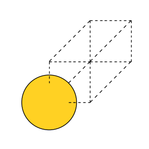
The last line opens the graphical user interface in which you can visually inspect the structures. Alternatively, the structures can be visualized using Python, which we do here for gold:

fig, ax = plt.subplots(figsize=(3, 3))
plot_atoms(atoms, ax)
ax.set_axis_off()

The bulk.db is an SQLite3 database in a single file:

$ file bulk.db
bulk.db: SQLite 3.x database

If you want to see what’s inside you can convert the database file to a json file and open that in your text editor:

$ ase db bulk.db --insert-into bulk.json
Added 0 key-value pairs (0 pairs updated)
Inserted 7 rows

or, you can look at a single row like this:

$ ase db bulk.db Cu -j
{"1": {
 "calculator": "emt",
 "energy": -0.007036492048371201,
 "forces": [[0.0, 0.0, 0.0]],
 "key_value_pairs": {"bm": 0.8392875566787444},
 ...
 ...
}

The json file format is human readable, but much less efficient to work with compared to a SQLite3 file.

Adsorbates

Now we do the adsorption calculations and store the results in the ads.db database:

path_to_ads_db = Path('ads.db')
ads_syms = ['C', 'N', 'O']
nlayers = [1, 2, 3]


def optimize_adsorbate(symb, alat, nlayer, ads):
    atoms = fcc111(symb, (1, 1, nlayer), a=alat)
    add_adsorbate(atoms, ads, height=1.0, position='fcc')

    # Constrain all atoms except the adsorbate:
    fixed = list(range(len(atoms) - 1))
    atoms.constraints = [FixAtoms(indices=fixed)]

    atoms.calc = EMT()
    opt = BFGS(atoms, logfile=None)
    opt.run(fmax=0.01)
    return atoms


# clean up if there is an old file
path_to_ads_db.unlink(missing_ok=True)
# again use context-manager
with connect(path_to_ads_db) as ads_db:
    for row in bulk_db.select():
        alat = row.cell[0, 1] * 2  # lattice constant
        symb = row.symbols[0]
        for nlayer in nlayers:
            for ads in ads_syms:
                atoms = optimize_adsorbate(symb, alat, nlayer, ads)
                myid = ads_db.reserve(layers=nlayer, surf=symb, ads=ads)
                if myid is not None:
                    ads_db.write(
                        atoms, id=myid, layers=nlayer, surf=symb, ads=ads
                    )

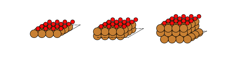
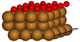
Let’s visualize the copper surfaces with 1, 2 and 3 layers that have oxygen adsorbed:

fig, axes = plt.subplots(ncols=3, figsize=(8, 2))
with connect(path_to_ads_db) as ads_db:
    for i, nlayer in enumerate(nlayers):
        atoms = ads_db.get(surf='Cu', ads='O', layers=nlayer).toatoms()
        atoms_sc = atoms * (4, 4, 1)
        plot_atoms(atoms_sc, axes[i], rotation='-70x,0y,0z')
        axes[i].set_axis_off()

We now have a new database file with 63 rows:

$ ase db ads.db -n
63 rows

These 63 calculations only take a few seconds with EMT. Suppose you want to use DFT and send the calculations to a supercomputer. In that case you may want to run several calculations in different jobs on the computer. In addition, some of the jobs could time out and not finish. It’s a good idea to modify the script a bit for this scenario. Therefore we added a couple of lines to the inner loop.

The reserve() method will check if there is a row with the keys layers=n, surf=symb and ads=ads. If there is, then the calculation will be skipped. If there is not, then an empty row with those keys-values will be written and the calculation will start. When done, the real row will be written into to the reserved row with id=myid. This modified script can run in several jobs all running in parallel and no calculation will be done twice.

In case a calculation crashes, you will see empty rows left in the database:

$ ase db ads.db natoms=0 -c ++
id|age|user |formula|pbc|charge| mass|ads|layers|surf
17|31s|jensj|       |FFF| 0.000|0.000|  N|     1|  Cu
Rows: 1
Keys: ads, layers, surf

Delete them, fix the problem and run the script again:

$ ase db ads.db natoms=0 --delete
Delete 1 row? (yes/No): yes
Deleted 1 row
$ python ads.py  # or sbatch ...
$ ase db ads.db natoms=0
Rows: 0

Reference energies

Let’s also calculate the energy of the clean surfaces and the isolated adsorbates and store them in the refs.db database:

path_to_refs_db = Path('refs.db')


def clean_surface_reference(symb, alat, nlayer):
    atoms = fcc111(symb, (1, 1, nlayer), a=alat)
    atoms.calc = EMT()
    atoms.get_forces()
    return atoms


# clean slabs
path_to_refs_db.unlink(missing_ok=True)
# connect to refs_db for writing
with connect(path_to_refs_db) as refs_db:
    # connect bulk_db for reading
    with connect(path_to_bulk_db) as bulk_db:
        for row in bulk_db.select():
            alat = row.cell[0, 1] * 2  # lattice constant
            symb = row.symbols[0]
            for nlayer in nlayers:
                myid = refs_db.reserve(layers=nlayer, surf=symb, ads='clean')
                if myid is not None:
                    atoms = clean_surface_reference(symb, alat, nlayer)
                    refs_db.write(
                        atoms, id=myid, layers=nlayer, surf=symb, ads='clean'
                    )

    # isolated atoms:
    for ads in ads_syms:
        atoms = Atoms(ads)
        atoms.calc = EMT()
        atoms.get_potential_energy()
        myid = refs_db.reserve(ads=ads)
        if myid is not None:
            refs_db.write(atoms, id=myid, ads=ads)

The previous code snippet saves those 24 reference energies (clean surfaces and isolated adsorbates) in a refs.db file. Suppose we want to extract the clean surfaces from the refs.db and store them in clean_surfaces.db. We could change the script and run the calculations again, but we can also manipulate the files using the ase db tool. First, we move over the clean surfaces:

$ ase db refs.db ads=clean --insert-into clean_surfaces.db
Added 0 key-value pairs (0 pairs updated)
Inserted 21 rows

If we want we can delete those from refs.db:

$ ase db refs.db ads=clean --delete --yes
Deleted 21 rows

Since this is only to demonstrate usage of the command line we will keep them.

Now we might want to extract the three atoms (pbc=FFF, no periodicity):

$ ase db refs.db pbc=FFF --insert-into isolated_atoms.db
Added 0 key-value pairs (0 pairs updated)
Inserted 3 rows

Finally, as we have not deleted anything these are the databases which we should have build so far:

$ ase db ads.db -n
63 rows
$ ase db refs.db -n
24 rows
$ ase db clean_surfaces.db -n
21 rows
$ ase db isolated_atoms.db -n
3 rows

Analysis

Now we have what we need to calculate the adsorption energies and heights:

# connect to ads_db for updating
with connect(path_to_ads_db) as ads_db:
    # connect to refs_db for reading
    with connect(path_to_refs_db) as refs_db:
        for row in ads_db.select():
            # atoms
            e_ads = refs_db.get(formula=row.ads).energy
            # clean surface
            e_clean = refs_db.get(
                surf=row.surf, layers=row.layers, ads='clean'
            ).energy
            ea = row.energy - e_ads - e_clean
            h = row.positions[-1, 2] - row.positions[-2, 2]
            ads_db.update(row.id, ea=ea, height=h)

Once run we can inspect the results for three layers of Pt:

$ ase db ads.db Pt,layers=3 -c formula,ea,height
formula|    ea|height
Pt3C   |-3.715| 1.504
Pt3N   |-5.419| 1.534
Pt3O   |-4.724| 1.706
Rows: 3
Keys: ads, ea, height, layers, surf

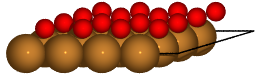
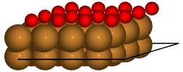
Finally, we can create more visually appealing figures using a renderer rather than ase.visualize.plot.plot_atoms(). These are saved as PNG files. See ase.io for more examples of rendering structures.

with connect(path_to_ads_db) as ads_db:
    for nlayer in nlayers:
        atoms = ads_db.get(surf='Cu', ads='O', layers=nlayer).toatoms()
        atoms_sc = atoms * (4, 4, 1)
        renderer = write(f'Cu{nlayer}O.pov', atoms_sc, rotation='-80x')
        renderer.render()

Note

While the EMT description of Ni, Cu, Pd, Ag, Pt, Au and Al is alright, the parameters for C, N and O are not intended for real work!